Intro Statistics for RPGs: Cyberpunk's Weird Dice Math

In yet another fit of pique, I got into running Cyberpunk Red. I'm enjoying the system, and now that my Castle Xyntillan game is back in rotation after holidays, I expect that I'll be able to run three games a week thanks to its low prep time.

A some months ago, I wrote Intro Statistics for RPGs: The Wheaton Dice Curse, since I had started my study of statistics. I have continued in force since then, and now I want to treat a much simpler topic

Today's lesson is a quick look at how Cyberpunk Red's dice mechanics create an unusual, discontinuous mass function.

Mass Functions

In statistics, the function which describes the probability of a given result of a discrete random variable is called the Probability Mass Function, or PMF. For continuous random variables, the term is Probability Density Function, PDF, but that's not what we're looking at today.

There are also Cumulative Mass Functions, which describe not the chances of getting any particular result, but the chances of being above a particular result. This is what we are looking to create.

Cyberpunk Red runs on d10s and d6s, though for our purposes, we're just interested in d10s. Dice are very simple random variables, ideally having a Uniform distribution. We're interested not in these objects, but in the chance of success they influence. However, Cyberpunk Red's dice are not simple uniform RVs. We'll get into the reasons why in a moment.

The cumulative mass function of Cyberpunk's dice takes this form:

P(X>x) = P(Y>(x-C))

Where X is the end result of the roll, the sum of C and Y, Y is a function describing the behavior of the dice, x is the integer Difficulty Value, and C is an integer constant, described below as the Base.

That's a whole lot of effort to say, 'the chance of beating a certain number is the same as the chance of getting more than the difference of the DV and your Base.' The use of specifying like this is that we can make some nice looking graphs that make it easier to see what's going on.

Background

In Cyberpunk, stats range from 2 to 8, with some options to raise them higher, such as with grafted muscles increasing the Body stat no further than 10. Skills range from 0 to 10. A starting character will have their best skills no higher than a 6. 

Cyberpunk Red's action resolution involves a dice roll that looks like 1d10+Base. Base is a combination of your skill rank and the stat associated with that skill. For example, shooting handguns is under the Handguns skill, which is attached to the Reflex stat. It's not unusual for starting characters to have a Base of 12 or more in a few skills which they use often.

That said, for our purposes, Base will also include situational modifiers, such as a -2 for not having the right tools, and also Luck. Luck is a stat, but instead of having associated skills or derived attributes, it serves as a pool of points which can be added to any roll. If you have a Luck score of 7, you have seven points to add to any of your rolls, which are regained only in the following session.

Non-Uniform Dice

Remember when I said above that Cyberpunk's dice aren't actually Uniform RVs? That's because of the dice explosion mechanic. Here's the PMF of rolling a certain number on Cyberpunk's d10.

In Cyberpunk Red, rolling a 10 is a critical success, and rolling a 1 is a critical failure. However, that does not mean that 10s automatically succeed and 1s automatically fail. When you roll either of those numbers, you roll the die again. If this was a critical success, you add the second roll to your total, while if it was a critical failure, you subtract. So you may roll a 1, then roll a 10, which means your total will be 9 fewer than your Base, including Luck and modifiers. 

This also means it is impossible to roll a 10 or a 1 on the dice alone.

It is actually possible to succeed even in the worst case by having a high enough Base and/or low enough Difficulty Value. And it is possible to fail in the best case with the inverse. 

But remember, unlike D&D's Difficulty Classes (DCs) which must be met or beaten to succeed on a task, Cyberpunk's Difficulty Values (DVs) must be beaten. Rolling a 13 on a DV13 check is a failure. 

The result is that, at certain points relative to the DV, increasing your base through Luck or decreasing it through negative modifiers actually has no effect on your chances of success.

For example, we have below the CMF of succeeding on a DV17 roll based on your Base. If your Base is a 16, then expending a point of luck to increase it to 17 is pointless*. Your chance of success is 90% either way. Likewise, there is no difference between a Base of 7 or 8. Your chance of success is 10%.

This is because of the dice explosion mechanic: if you have a DV17 check and a Base of 16, you will get an 18 or higher on any roll of a 2 or more, 90% chance. If you roll a 1, then you will end up subtracting at least 1 point from that, such that it is impossible to roll a total which is exactly 1 above your base. But if you have a Base 17, you still need to roll a 2 or better; if you roll a 1, you will end up subtracting at least 1, at best getting you to 17, and likely lower.

Similarly, this means that Base scores greater than the DV and less than 10-DV have greatly diminishing returns from modifiers. If you're in the main body range of (DV-9) =< x =< (DV-1) then increases and decreases to other points in that range result in 10% changes to success rate for each point of modification. But just beyond that range, the probabilities plateau, and beyond that, each point buys just a 1% increase or decrease in success rate.

The simple version of all this for use at the table is that it's not worthwhile to push your Base beyond DV-1 using a limited resource. You're already at 90%, further improvements are a tenth as valuable as they would be in riskier rolls. 

*The exception to this is in cases where not only succeeding, but beating the DV by a certain margin, matters. Ordinarily, this is not the case, but Autofire rolls in Cyberpunk Red deal different amounts of damage based on how much you beat the DV.

The Cumulative Relationship

Do the two graphs above look weirdly similar somehow? That's because the Cumulative Mass Function, CMF, is the sum of the PMF previous to that point. If we were dealing with CDFs and PDFs, the continuous version, then the relationship is not one of sum, but of integral and derivative. That, and the PMF is centered around the mean of 5.5, while the CMF is shifted to the right owing to the position of the DV. 

--------------------

If you enjoyed what you read here, make sure to follow the blog and share the post! Leave your comments down below. Until the next post, have an excellent week!

Intro Statistics for RPGs: The Wheaton Dice Curse

I watched Critical Role when I first got into RPGs, though I didn't get too far into the series. Still, I remember the episodes guest-starring Will Wheaton, and the 'Wheaton Dice Curse', his tendency to get very bad rolls, including far more natural 1s than should be, well, natural. I looked it up, and found the folks over at Critical Role Stats (which is a thing that exists, apparently) had already addressed it, although their analysis was very shallow to me. 

Given that I took an intro stats course this past quarter, I thought it would be worthwhile to give the topic a deeper look, and in doing so both refresh my own knowledge and teach y'all some basic stats. 

Today's lesson will be introducing variance, Bernoulli and Binomial distributions, p-values, elementary hypothesis testing, z-scores and the CLT. I'll be using RStudio, a free dev environment for the R programming language. If you have it on your computer, I'll put down the code as we go so you can follow along. Otherwise, I'll just show my work, and you can take my word that the program spits out what it does. For anyone wanting to learn some basic stats on their own time, I recommend OpenIntroStats, which is a free digital textbook. It's what I used in my college class, it's well written and clear, and has  ton of practice problems. 

Examining the Dataset

The dataset is Wheaton's rolls over two Critical Role sessions, in which he rolled 54 times. Not great, but I've used smaller, and the measurements we'll be using take scale into account. CR Stats made a histogram of the frequency of each number on the d20, from Wheaton's 54 separate rolls. 

This is pretty far off our expected frequencies. In particular, the number of natural 1s and 2s are way off. We'll copy down the numbers into a list, and apply the c() function to turn them into a vector. Then we'll assign it to an easy to remember and convenient name to call it later. We can use the var() function on our dataset to return the variance value. Then we can take the square root of the variance to find the standard deviation.

x<- c(1, 1, 1, 1, 1, 1, 1, 1, 1, 1, 2, 2, 2, 2, 2, 2, 2, 3, 3, 3, 3, 4, 4, 4, 4, 5, 6, 6, 6, 6, 6, 7, 7, 8, 8, 9, 9, 9, 9, 11, 11, 12, 13, 13, 14, 14, 14, 15, 15, 17, 18, 19, 19, 20)

var(x)

Returns 32.90566, standard deviation 5.736346. Variation and standard deviation are both sequence invariant, so you could put it in the original order of rolls or order them like this, and get the same answer. However, these measures are sensitive to scale; if you maintained the same ratio of rolls, but over a larger number of rolls, the variance would be lower. Interestingly, the variance of this dataset is lower than that of an expected set of similar length. It's not just biased towards lower numbers, it's more concentrated there are well.

Natural 1s

Predicting natural 1s is a Bernoulli variable. Bernoulli variables are those which can either fail or succeed a criterion with a certain probability, on a set number of trials. The classic Bernoulli variable is the fair coin flip, which is either heads or tails with a probability of 1/2. 

Our d20, landing on either a natural 1 (success) or anything else (a failure) is a Bernoulli 1/20 variable, Bern~(.05). So, how far out of line are Wheaton's natural 1s? Well, our expected number of natural 1s is simply the number of trials times the probability, so on 54 trials, we should expect 2.7 natural 1s. Instead, we get 10.

10 instead of 2.7 is a big difference, but how far off is it if Wheaton just had bad luck on this set of rolls? Here we'll do some basic hypothesis testing.

Hypothesis Testing the Curse

Hypothesis testing is where we set some hypotheses and a test metric for them with a preselected alpha-level, the threshold for p-values. In this case, we're going to perform a hypothesis test on our number of natural 1s, to see how rare this outcome really is under our null hypothesis.

Our null hypothesis, H0, is our assumption that the die is fair and Wheaton's rolls are luck alone. Our alternate hypothesis, HA or H1, is that Wheaton is, in reality cursed. First, we're going to select our alpha level. The alpha level is a number between 0 and 1 that reflects the likelihood of finding an example more extreme than our current observation by sheer chance. The lower the number, the less you expose yourself to false rejections.

A Digression on P-Values

You've likely heard of statistical significance, and linked it to a p-value less than .05. This means that if the observed p-value is less than .05, you are confident enough to reject the null, and the finding is considered 'statistically significant'. If not, you are unwilling to, and it isn't. What the .05 value reflects is a tolerance for false rejections 1 in 20 times. That is, if you had 20 studies with a p-value of .05, you'd expect one to be wrong. If you set your p-value to .01, you're expecting a false rejection by pure chance 1 in 100 times. 

The expected p-values are going to differ based on the size and rarity of the effect you're trying to measure; in high-energy physics, you're routinely looking at p-values on the order of 10^-6 or -7, due to the regularity of the systems being studied. In more chaotic fields, like biology, you'll get laughed out of the room if you have a p-value that small since very few experiments in the field have that kind of sensitivity and it means you probably screwed up. In the social sciences, even p<.05 is often too generous.

[This is a very basic explanation, and real life is quite different. Your p-value is only valuable if you've adequately controlled for confounders; if you haven't, you probably have some systematic bias in your data, and your study might be worthless if your mistake was really bad. P-hacking, which is the act of modifying your p-values by messing with your experiment, is rampant, especially in the social sciences, and far more than 1 in 20 such studies fail to replicate. If you want to dig in more, I recommend this somewhat technical post and this much more entertaining less technical post]

Back to the Curse

How precise do we want to be? Well, dice rolling is mechanical physics, and while using math to determine which face will come up is very complex, the effects are regular and, like coin flipping, we expect the chaos to even out. There's also the possibility of the dice in use being biased towards lower numbers. But the hypothesis we're looking to test here is whether or not Will Wheaton is cursed, and this is going to depend a lot based on how much you believe in curses. So we'll use multiple confidence levels to illustrate.

Alice is a big believer in witchcraft, hexes and curses, and thinks Wheaton got what was coming to him for his portrayal of Wesley Crusher. Still, she's not certain this is the effect of a curse, so she'll put forward an alpha level of .05. 

Bob is a little superstitious, but is much less bullish on the topic than Alice. He'll put forward an alpha level of 1 in a thousand, .001. 

Cassandra is a hard-nosed secularist, and disdains the very notion of a curse. She puts forward an alpha level of one in ten million, .0000001. She doesn't expect to be convinced. 

And before we go forward, let's formalize our hypotheses.

H0, the null: Will Wheaton's d20s are regular polyhedral objects, and rolling natural 1s on them is adequately described by Bern~(.05).

HA, the alternate: Will Wheaton is cursed, and as a result his dice roll natural 1s with a probability greater than .05. 

Now to set up the actual measurement. Bernoulli variables are neat, but they're a measure focused around single observations. How do we analyze a collection of many Bernoulli variables?

We use the Binomial distribution. There's a few criteria we need to pass before using the Binomial is valid; the trials have to be independent, meaning that each die roll has no effect on another, the number of trials has to be fixed, each must be classified as either a success or failure, and must have the same probability across the trials. So long as the curse modifies the probability across the whole on a consistent basis, we're good.

The code looks like this: pbinom(observed value, number of trials, success probability)

We'll also add another argument at the end, lower=F, which means we're looking at the upper end of the distribution. It's equivalent to using 1-pbinom(), but it looks neater. We'll also use binomial definitions for mean and standard deviation to find those for later.

μ = np = .05*54 = 2.7

sd=sqrtn*(p*(1-p)) = sqrt(54*.05*(.95)) = 1.601562

Observed value = 10

pbinom(10, 54, .05, lower=F) 

Returns 6.315881e-05, or .00006315881

Also, if you don't have RStudio, you can still find this using a calculator, or even get pretty close with a pen and paper. We established that the mean in 2.7, and our observed value is 10. 10-2.7 = 7.3, and we can divide this by our standard deviation to get a value of around 4.5. This means that our observed value is about 4.5 standard deviations away from our estimate. You might hear this called '4.5 sigma', it means the same thing.

However you do it, you find a very big difference. 4.5 Sigma is WAAAY out of the ordinary, and the 6.315881e-05 figure tells us that the chances of getting this by chance is around 6 in a hundred thousand. 

Cassandra is unimpressed. It's less likely than she expected, but nowhere near unlikely enough to challenge her low prior belief in curses.

Bob and Alice's estimates, on the other hand, are burst open. They now believe that Will Wheaton is cursed, and have a fancy-shmancy number to show for it.

Testing the Mean

Mind you, all we've shown here is that natural 1s are occurring with more frequency than should be expected. We can do the same for every other number if we want. The natural 2s are also interesting, and with the work done above, finding the answer for that roll by either method should be trivial. I've included the answer at the bottom. 

But that's just certain rolls. A more common form of hypothesis testing looks at the mean of these distributions. We can also look at these with similar methods. When hypothesis testing means, the hypotheses look like this.

H0: μ = expected mean (10.5 in our case)

HA: μ = greater or less than expected mean, depending on investigator belief.

The null is sometimes formalized as (observed mean) - (expected mean) = 0, which better fits the normal distribution which is most often used for this.

Expected mean for a null distribution: 10.5

mean(x) = 7

Huh. 7 exactly. So, if the true mean should be 10.5, how unlikely is it we get to 7 by chance instead? I'll quickly calculate this out using a method of normal approximation called the Central Limit Theorem and the pnorm() function, since we're looking at probabilities on the normal distribution instead. We'll use a formula to find a value called the z-score, which is stabilized to the standard normal distribution. Note also that we'll use the standard deviation we calculated at the start of the post. This can be risky with small sample sizes, since it might be calculated from unusual data, but as a rule of thumb it's usually permissible to do so with sample sizes greater than 30, and here we have 54 trials.

P(μ < 7) = P( z <((7-10.5)/(5.736346/sqrt(54)))) = P(z < -4.483628) 

We then take pnorm(-3.84311), without adding anything else, since we're looking at the lower bound and the z-value is made for the standard normal, and find...

pnorm(-4.483628) = 3.669227e-06

Another long shot, even further off than our estimate for the natural 1s, around 36 in 10 million. Though I'm not confident enough to talk about the general shape of the curse, Alice and Bob certainly have reason to believe in the effect.

In conclusion, if you have a prior belief in curses and hexes around or greater than the order of 10e-5, you have substantial reason to believe that the Wheaton dice curse, even from this single set of games in isolation, let alone a more general trend claimed by Wheaton. 

Oh, and if you've read through this post with a consistent sense of disgust that I'm even applying statistics to something so obviously ridiculous, I recommend you look into the natural control group that is parapsychological research as a similar touchstone. If a mediocre first year stats student can pull a 10e-5 order effect out of a tiny dataset relating to an absurd concept, you might consider being more skeptical about other random statistics you read about on the internet.

I hope you all enjoyed the post! I'm not 100% sure about all the numbers here, especially in the correspondence between the sigmas and the probabilities, but it's about right. If you have any questions, corrections, or want to see more like this in the future, be sure to write me down in the comments below! Until then, I'm in the middle of two family birthdays and have to get back to getting wasted.

pbinom(7, 54, .05, lower=F)

Returns 0.005180117

4.3/1.601562

Returns 2.684879 sigma

Volume of a 4-D pyramid in a 4-D cube

If you clicked on this post wondering how I'm stretching pyramids and higher dimensions to apply to old-school roleplaying, I'm afriad you will be disappointed. In addition to role-playing, I'm an amateur mathematician in real life, and recently made my first original proof (not original in that nobody has ever shown it before, moreso that I didn't look it up on Wikipedia). This blog will today, and intermittently in the future, become a low-level mathematics blog.

If your first reaction to mentions of mathematics is, 'Ugh, math is stupid and boring,' then I invite you to read A Mathematician's Lament by Paul Lockhart, who agrees with your assessment and shows why math is actually fun.

Everything from this point on is very basic, involving very little computation, and what there is is only trivial integration, which you need not understand to get the proof. It, like most proofs in basic mathematics, can be shown with natural language and diagrams. Now, on with the show.

-----------------------------

Question: What ratio of the volume of a 4-D cube is taken up by the largest 4-D pyramid that fits inside it? If possible, what is the general expression for the same problem on all dimensions n?

Guess: Without working out a proof, I posit that the answer is likely to be ¼. This is extrapolated from the n=2 and n=3 versions of the question, for which the answers are ½ and ⅓ respectively. These facts are embodied in the formulas for area and volume of a triangle and pyramid: lh/2 and lwh/3, respectively.

Reasoning
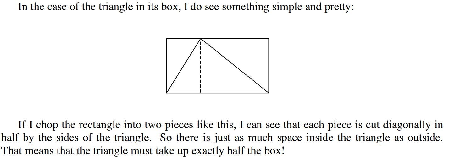
In his open letter A Mathematician's Lament, Paul Lockhart gives an elegant visual proof of the n=2 answer. Drawing a line through the top vertex of the triangle gives us two new rectangles, each of which is clearly half filled by two new triangles. Thus, the whole triangle is half the whole rectangle.



Let us assume from this point that all squares, cubes and hypercubes in our examples are in their unit form; all sides equal 1.

While the 3-D version is subject to a similar visual proof, by splitting it into 4 segments along the z-axis centered around the top vertex, it is much less useful, as these objects are much less obviously one third of their respective cuboids. If the 3-D visual proof is not self-evident, we may assume that the 4-D version will be less so.

Back to the drawing board.

Idea: We can reach ‘up’ a dimension without straining human intelligence by using time as the 4th dimension.

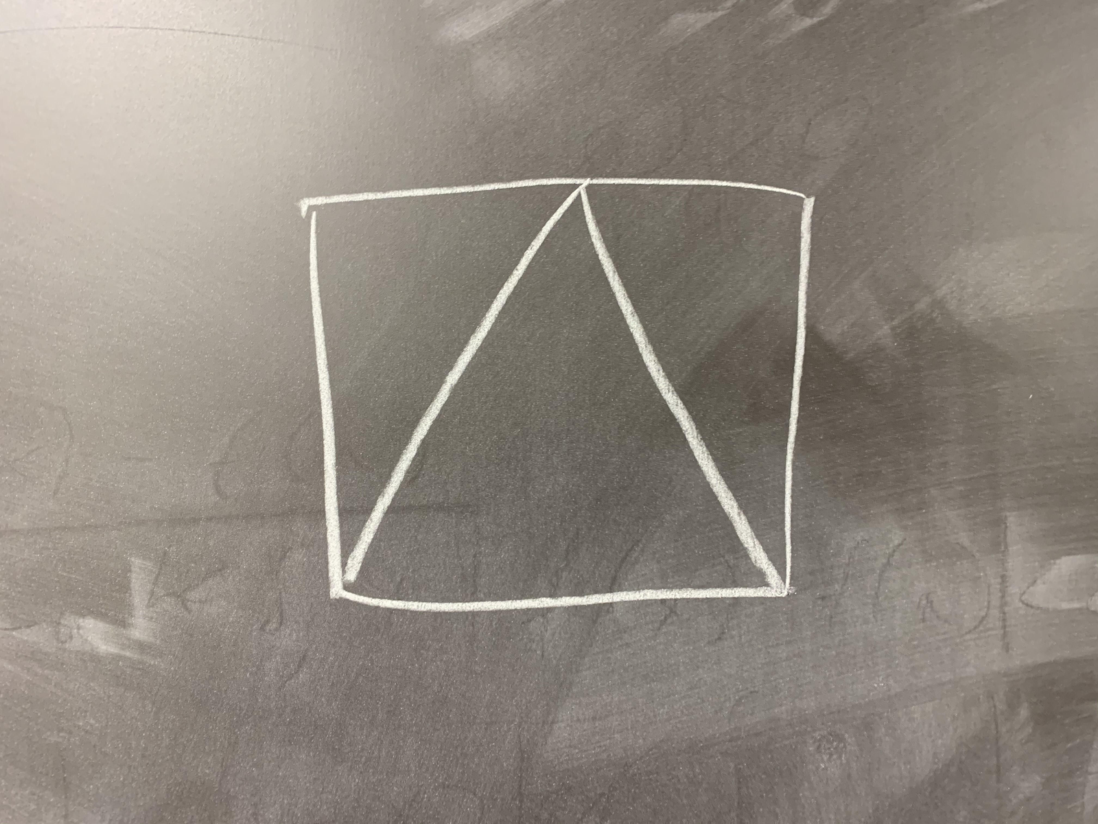
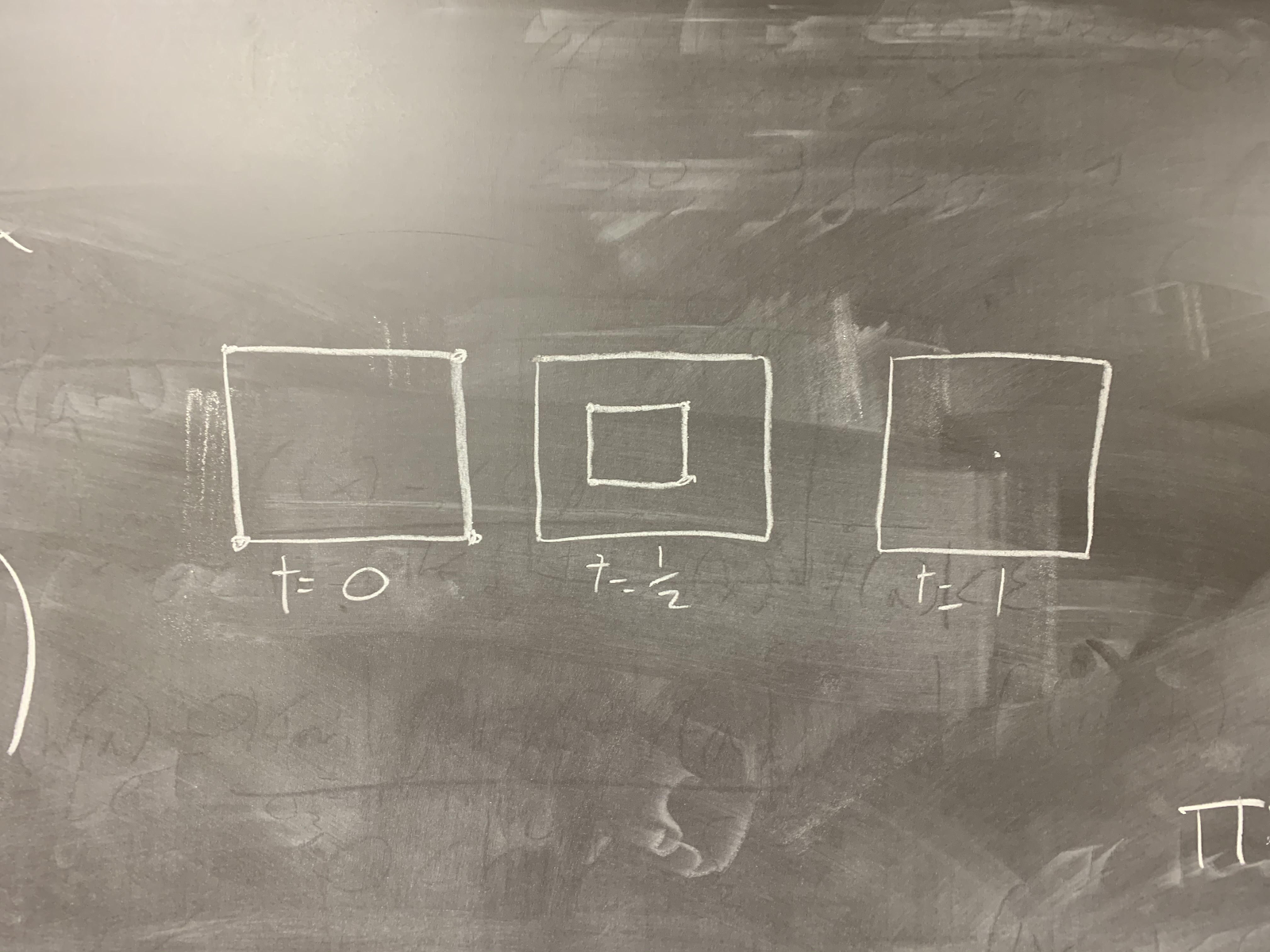
Proof of concept in 2-D: We can adequately represent the 2-D version of this problem using only a single spatial dimension, and one temporal dimension. Consider that the ‘base’ of our 2-D pyramid is a line, which coincides exactly with the bottom side of the square.



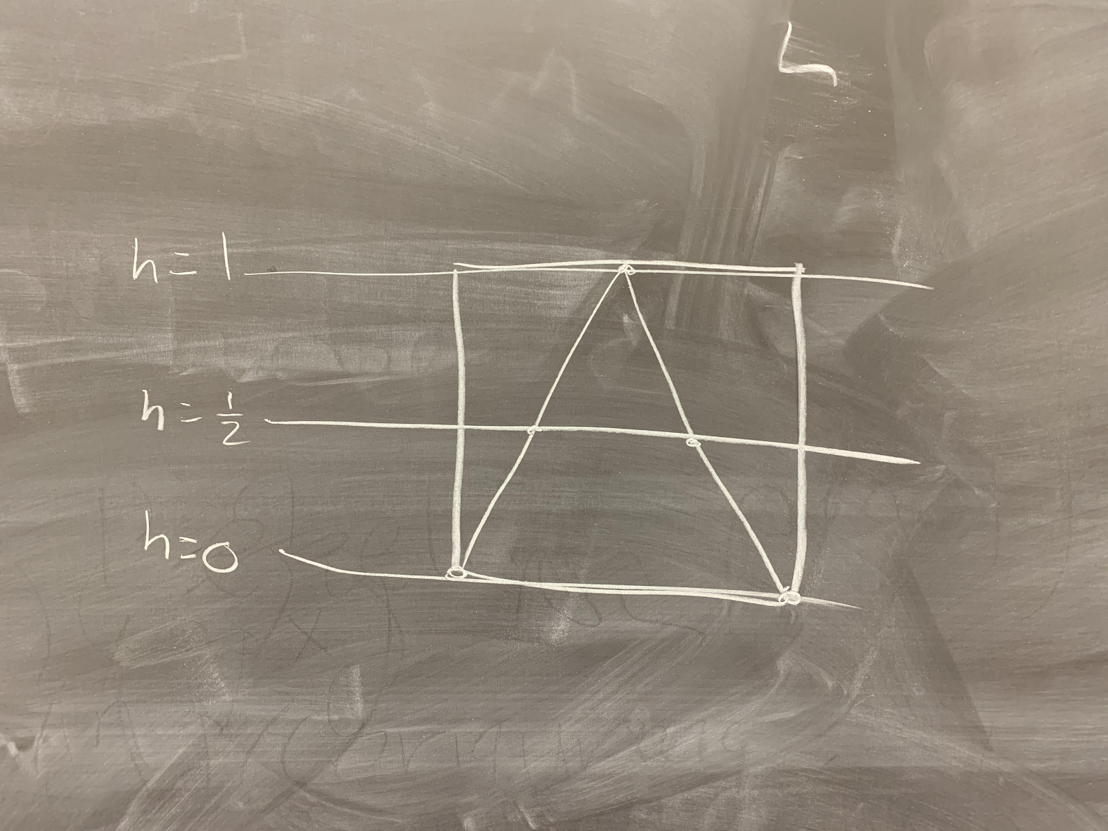
We may draw horizontal lines across the figure, and in the process take a cross-section of the triangle. This cross-section takes the form of points on a line. Consider the cross sections taken at the heights h=0, h=½ and h=1



The first has the triangle points coinciding exactly with the bottom corners of the square. The second places them at ¼ and ¾ on the line [0, 1], leaving exactly half the line between them. Finally, the third has a single point the center of the line; the top vertex of the triangle.

But what use are these? These segments, when laid out, are precisely the 1-D representations of the 2-D figure in the temporal dimension, at t=0, t=½, t=1.



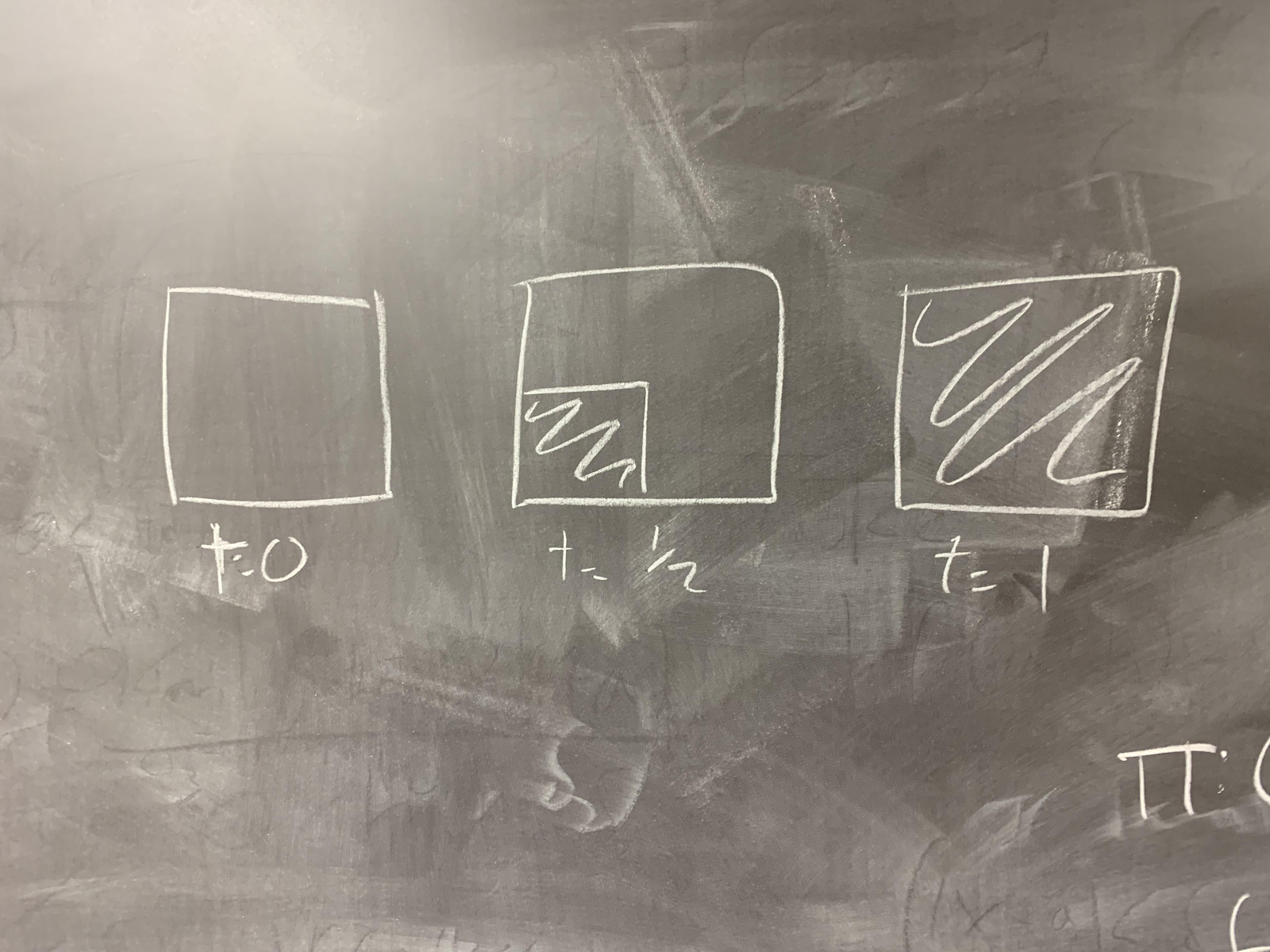
Proof of concept in 3-D: We may expand to the 3-D version, replacing the height dimension once again with time. The cross-sections are now taken by horizontal xy planes at z=t, and the pyramid is adequately represented by a shrinking square set within the static square of the cube.



Proof of concept in 4-D: The method holds, and so we export to the fourth dimension. The cross sections now take the form of growing cubes, set within static cubes. These, of course, represent cross-sections taken of the hyper-pyramid by R^3 spaces in R^4 space (my non-specialist vocabulary breaks down here, but the metaphor yet functions) at א=t.

(I use the א though it has other meanings in higher mathematics for two reasons. First, it allows me to flex my usage of a Hebrew keyboard, a rare event indeed. Second, on such a keyboard, א is in fact tied to the t key, which I consider kabbalistically appropriate).



Calculation
Now that we have a robust model for pyramids in cubes in higher dimensions, how can we calculate their exact volume? My calculus professor, Shiva Chidambaram, encouraged me to try using integration to solve the problem, since we are currently learning multivariable integration. However, he also informed me that there is a simpler proof that requires only single variable integration.

Going back to the 2-D example, we can backfit a simple solution.

Our slope for the pyramid, as shown here, is y=x. Replacing height with time, and redrawing our triangle for simplicity, we can show simply that f(t)=x.



The general integral is trivial: F(t)=(x^2)/2. We can integrate on our bound of [0, 1] with similar ease, and the result is ½, as expected.

Scaling up to 3-D, we find ourselves now calculating the volume of the pyramid from square cross-sections. By redrawing the examples shown previously, it is clear that the area is given by f(t)=x^2.



Our integral, similarly trivial, is (x^3)/3, and on [0, 1], integrates to ⅓.

Having shown the above, I am confident in scaling this approach up to 4-D. The size of the cross section cubes is given by f(t)=x^3, the integral by F(t)=(x^4)/4, and on [0, 1] is equal to ¼. This confirms my original guess. Score one for intuition.

Quod Erat Demonstrandum

Further, I am confident in scaling this approach up to all dimensions n. For the volume of an n-dimensional pyramid set in an n-dimensional cube, the volume may be given as (s^n)/n, where s equals the length of the cube’s sides, and the ratio of volume is simply 1/n.

So for a 3-D cube of side length 4, the pyramid’s volume is 64/3. For a 5-D cube of side length 3, the pyramid’s volume is 243/5, and so on.

QED

Remaining question

All this begs the question. Is there a simpler proof that the one outlined above, preferably one that does not require even trivial integration? That is yet to be seen, and I refuse to look up the answer.

Musical observation

Mozart’s Don Giovanni is perfectly adequate listening material for composing mathematics. Madamina (tin tin tin) il catalogo e questo...